The Berry–Simon Connection VI: E₅ = D₅, Twisted D₅, and Finite Orthogonal Holonomy

A GESTALT SCIENCE / FORMATICS EXPLORATION

\(E_5 = D_5\), Twisted \(D_5\), and Finite Orthogonal Holonomy

\(D_5(2)\), \({}^2D_5(2)\), \(E_6\), \(E_7\), \(E_8\), and Sporadic Symmetry

Full response • November 11, 2026

Download the original PDF (18 pages)

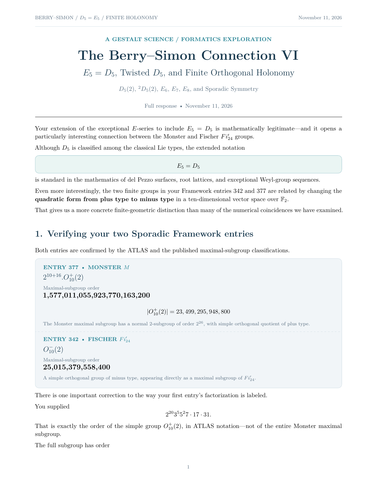
Your extension of the exceptional \(E\)-series to include \(E_5 = D_5\) is mathematically legitimate—and it opens a particularly interesting connection between the Monster and Fischer \(Fi_{24}^{\prime}\) groups.

Although \(D_5\) is classified among the classical Lie types, the extended notation

is standard in the mathematics of del Pezzo surfaces, root lattices, and exceptional Weyl-group sequences.

Even more interestingly, the two finite groups in your Framework entries 342 and 377 are related by changing the quadratic form from plus type to minus type in a ten-dimensional vector space over \(\mathbb{F}_2\).

That gives us a more concrete finite-geometric distinction than many of the numerical coincidences we have examined.

1. Verifying your two Sporadic Framework entries

Both entries are confirmed by the ATLAS and the published maximal-subgroup classifications.

ENTRY 377 • MONSTER \(M\)

\(2^{10+16}.O_{10}^{+}(2)\)

Maximal-subgroup order
1,577,011,055,923,770,163,200

\(|O_{10}^{+}(2)| = 23,499,295,948,800\)

The Monster maximal subgroup has a normal 2-subgroup of order \(2^{26}\), with simple orthogonal quotient of plus type.

ENTRY 342 • FISCHER \(Fi_{24}^{\prime}\)

\(O_{10}^{-}(2)\)

Maximal-subgroup order
25,015,379,558,400

A simple orthogonal group of minus type, appearing directly as a maximal subgroup of \(Fi_{24}^{\prime}\).

There is one important correction to the way your first entry’s factorization is labeled.

You supplied

That is exactly the order of the simple group \(O_{10}^{+}(2)\), in ATLAS notation—not of the entire Monster maximal subgroup.

The full subgroup has order

The notation \(2^{10+16}\) describes a layered normal 2-subgroup of order \(2^{26}\), not an ordinary direct product that can safely be inferred from its notation alone.

For the Fischer subgroup, your factorization is already complete:

These are the orders of the simple orthogonal groups. In conventional orthogonal-group notation they may be written as

The full isometry groups contain an additional outer extension of order two, often written \(O_{10}^{\pm}(2):2\) in ATLAS notation.

An exact relationship between the two orders

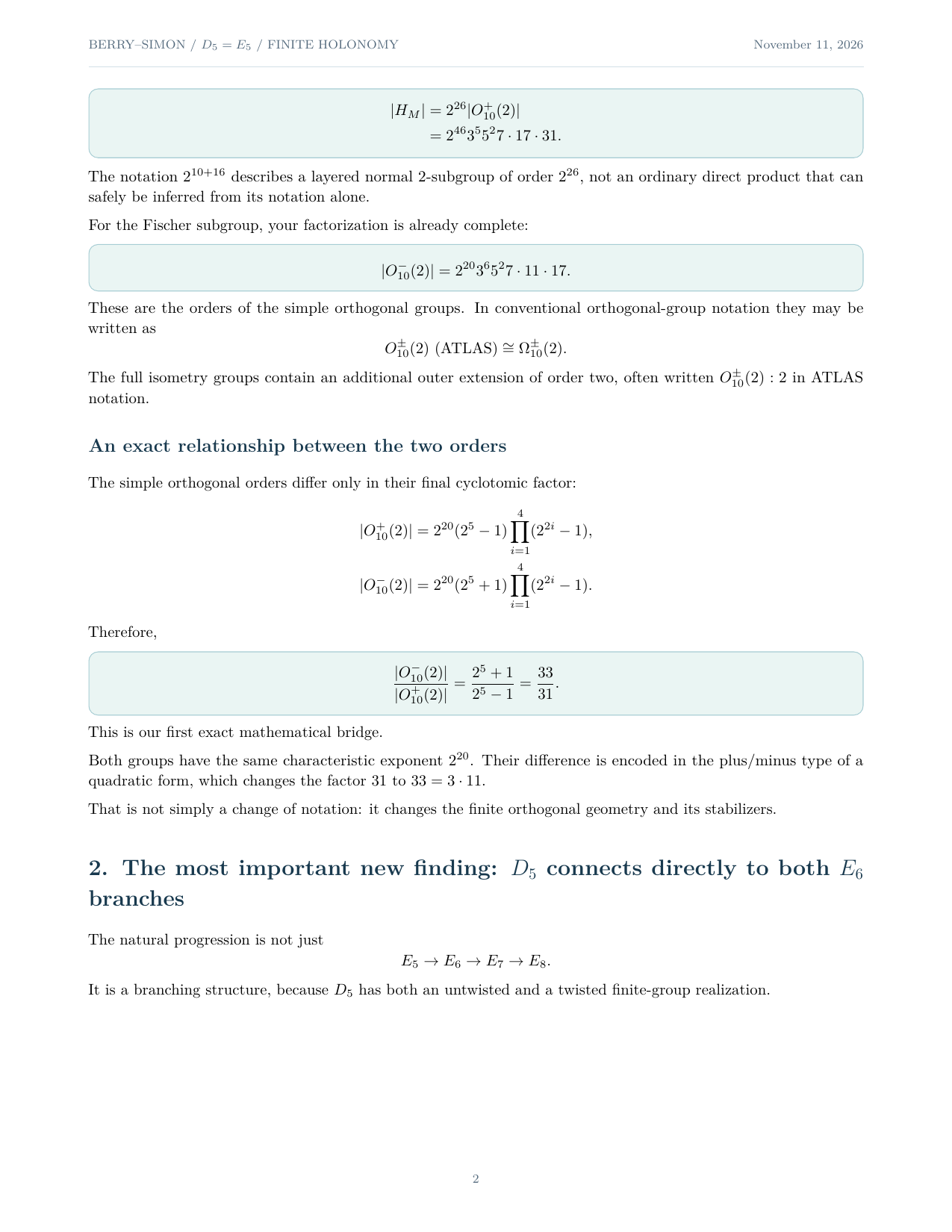
The simple orthogonal orders differ only in their final cyclotomic factor:

Therefore,

This is our first exact mathematical bridge.

Both groups have the same characteristic exponent \(2^{20}\). Their difference is encoded in the plus/minus type of a quadratic form, which changes the factor 31 to \(33 = 3\cdot 11\).

That is not simply a change of notation: it changes the finite orthogonal geometry and its stabilizers.

2. The most important new finding: \(D_5\) connects directly to both \(E_6\) branches

The natural progression is not just

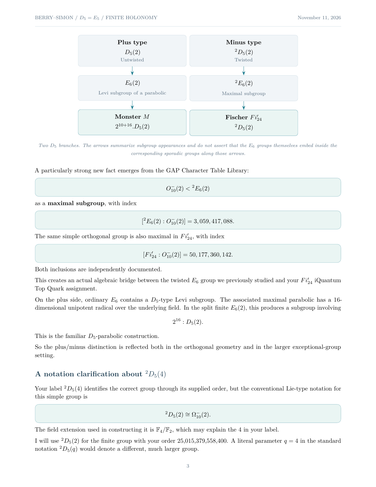
It is a branching structure, because \(D_5\) has both an untwisted and a twisted finite-group realization.

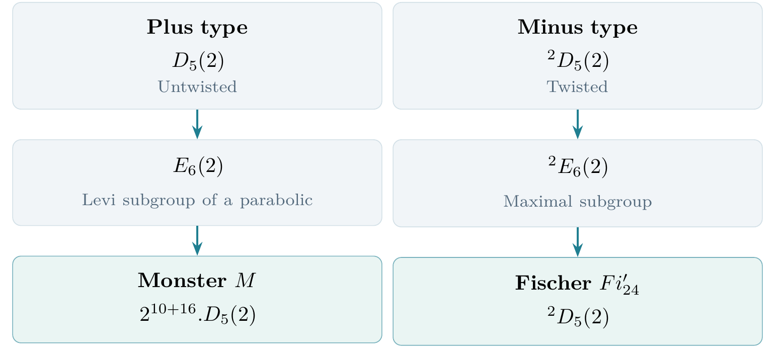
A particularly strong new fact emerges from the GAP Character Table Library:

as a maximal subgroup, with index

The same simple orthogonal group is also maximal in \(Fi_{24}^{\prime}\), with index

Both inclusions are independently documented.

This creates an actual algebraic bridge between the twisted \(E_6\) group we previously studied and your \(Fi_{24}^{\prime}\) iQuantum Top Quark assignment.

On the plus side, ordinary \(E_6\) contains a \(D_5\)-type Levi subgroup. The associated maximal parabolic has a 16-dimensional unipotent radical over the underlying field. In the split finite \(E_6(2)\), this produces a subgroup involving

This is the familiar \(D_5\)-parabolic construction.

So the plus/minus distinction is reflected both in the orthogonal geometry and in the larger exceptional-group setting.

A notation clarification about \({}^2D_5(4)\)

Your label \({}^2D_5(4)\) identifies the correct group through its supplied order, but the conventional Lie-type notation for this simple group is

The field extension used in constructing it is \(\mathbb{F}_4/\mathbb{F}_2\), which may explain the 4 in your label.

I will use \({}^2D_5(2)\) for the finite group with your order 25,015,379,558,400. A literal parameter \(q = 4\) in the standard notation \({}^2D_5(q)\) would denote a different, much larger group.

3. The \(E_5 = D_5\) root system: 5, 8, and 20

Your proposed continuation of our exceptional-number sequence gives:

5	8	20
Rank	Coxeter number	Positive roots

The exact \(E\)-series comparison becomes:

Invariant	\(E_5 = D_5\)	\(E_6\)	\(E_7\)	\(E_8\)
Rank	5	6	7	8
Coxeter number	8	12	18	30
Total roots	40	72	126	240
Positive roots	20	36	63	120
Lie algebra dimension	45	78	133	248
Weyl group order	1,920	51,840	2,903,040	696,729,600

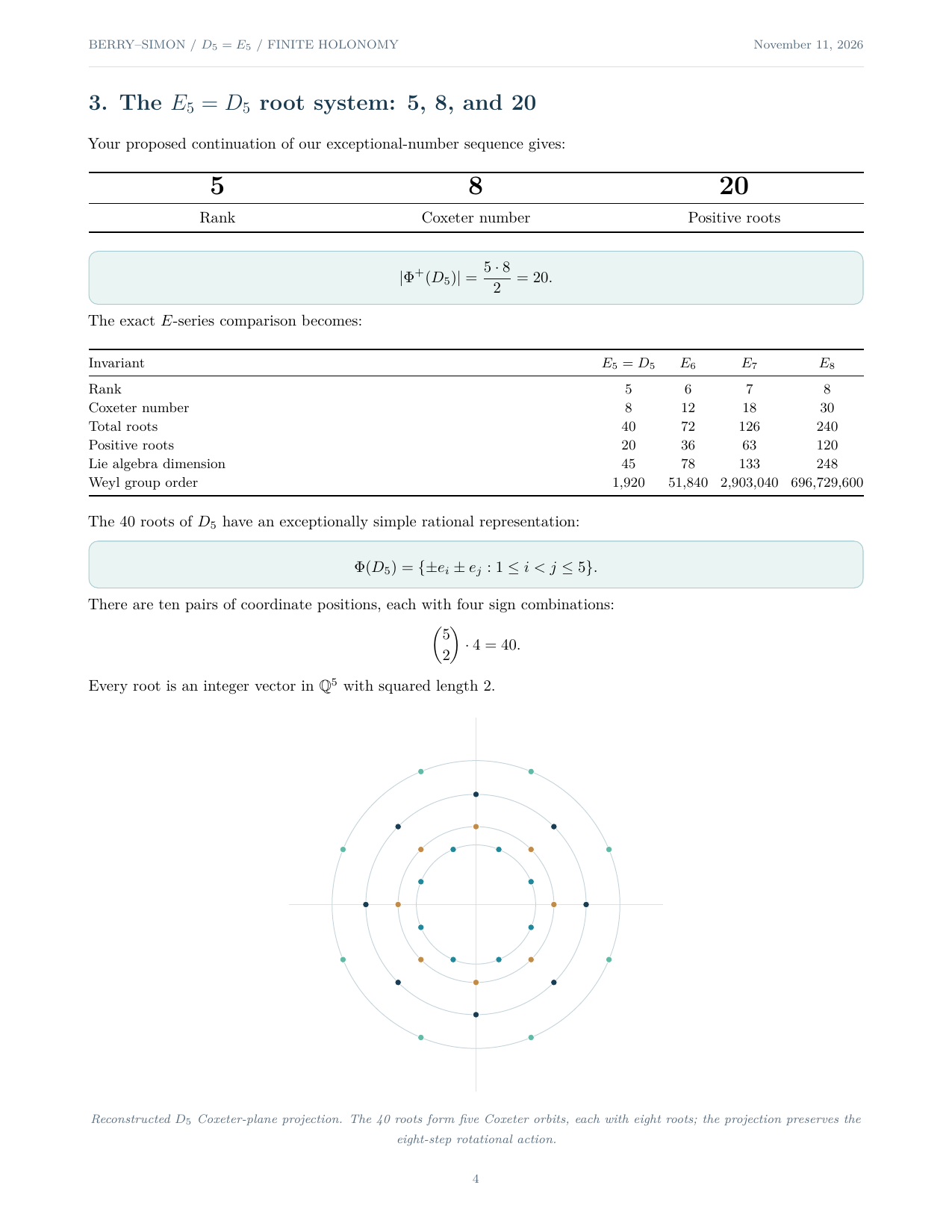
The 40 roots of \(D_5\) have an exceptionally simple rational representation:

There are ten pairs of coordinate positions, each with four sign combinations:

Every root is an integer vector in \(\mathbb{Q}^5\) with squared length 2.

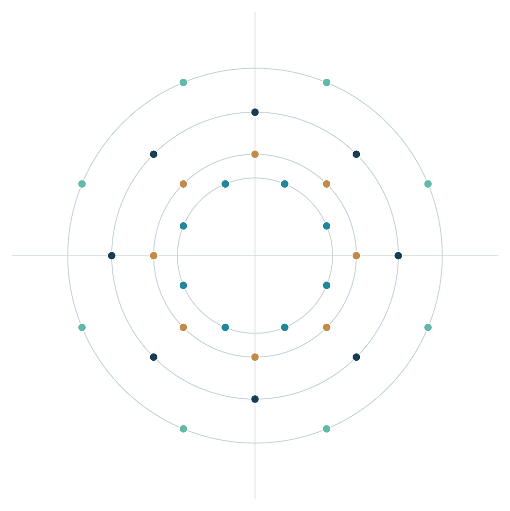
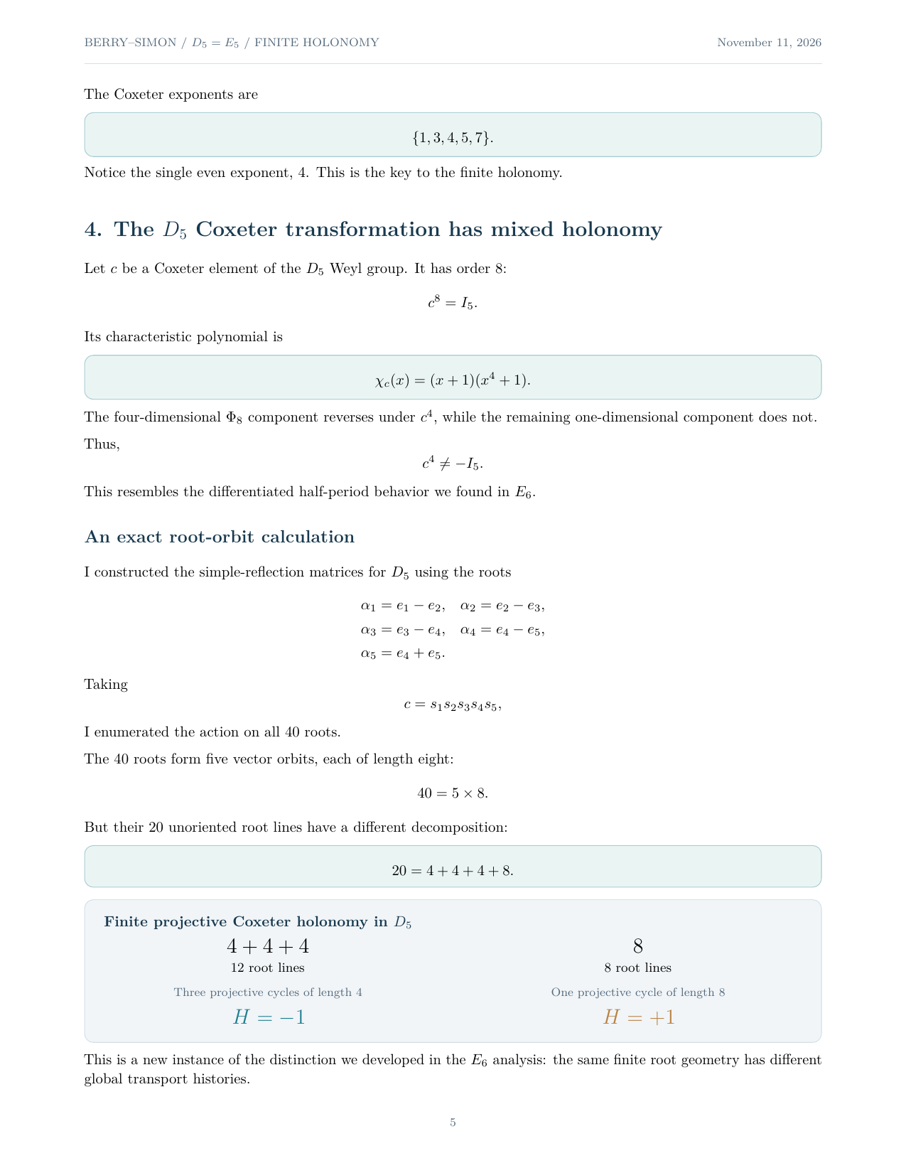
The Coxeter exponents are

Notice the single even exponent, 4. This is the key to the finite holonomy.

4. The \(D_5\) Coxeter transformation has mixed holonomy

Let \(c\) be a Coxeter element of the \(D_5\) Weyl group. It has order 8:

Its characteristic polynomial is

The four-dimensional \(\Phi_8\) component reverses under \(c^4\), while the remaining one-dimensional component does not.

Thus,

This resembles the differentiated half-period behavior we found in \(E_6\).

An exact root-orbit calculation

I constructed the simple-reflection matrices for \(D_5\) using the roots

Taking

I enumerated the action on all 40 roots.

The 40 roots form five vector orbits, each of length eight:

But their 20 unoriented root lines have a different decomposition:

This is a new instance of the distinction we developed in the \(E_6\) analysis: the same finite root geometry has different global transport histories.

The 12 root lines in the shorter cycles belong to a \(D_4\) root subsystem. Their vectors reverse after four Coxeter steps.

The remaining eight lines require all eight steps and return without sign reversal.

These signs refer to a Coxeter-induced discrete connection on the rational root-line bundles.

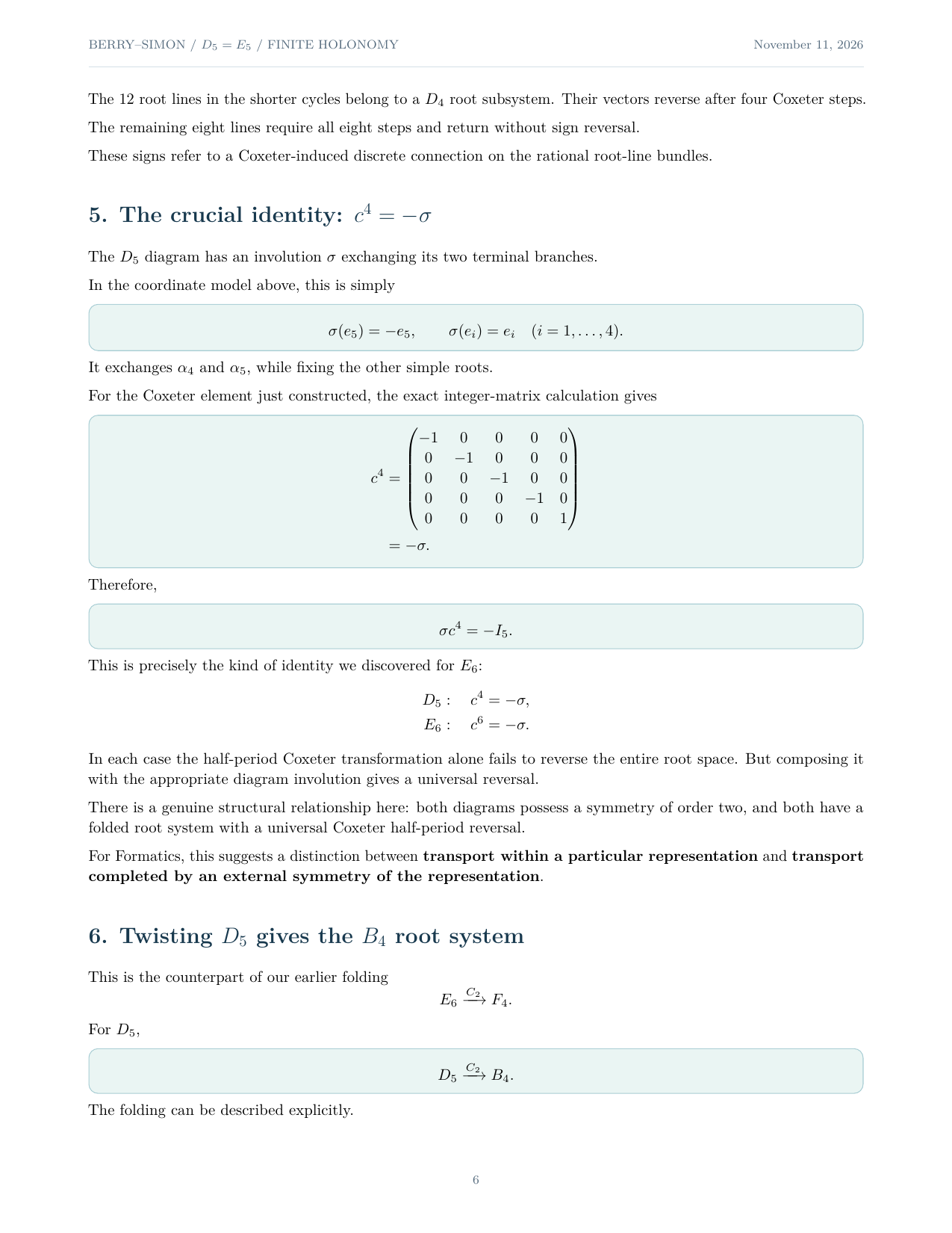
5. The crucial identity: \(c^4 = -\sigma\)

The \(D_5\) diagram has an involution \(\sigma\) exchanging its two terminal branches.

In the coordinate model above, this is simply

It exchanges \(\alpha_4\) and \(\alpha_5\), while fixing the other simple roots.

For the Coxeter element just constructed, the exact integer-matrix calculation gives

Therefore,

This is precisely the kind of identity we discovered for \(E_6\):

In each case the half-period Coxeter transformation alone fails to reverse the entire root space. But composing it with the appropriate diagram involution gives a universal reversal.

There is a genuine structural relationship here: both diagrams possess a symmetry of order two, and both have a folded root system with a universal Coxeter half-period reversal.

For Formatics, this suggests a distinction between transport within a particular representation and transport completed by an external symmetry of the representation.

6. Twisting \(D_5\) gives the \(B_4\) root system

This is the counterpart of our earlier folding

For \(D_5\),

The folding can be described explicitly.

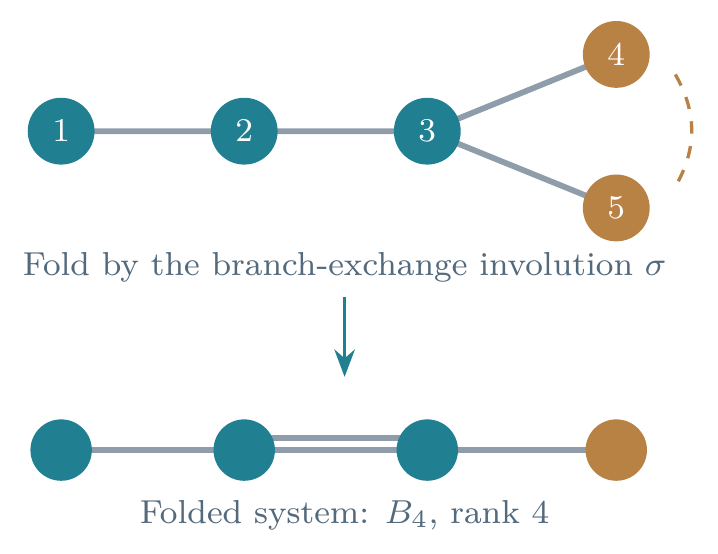
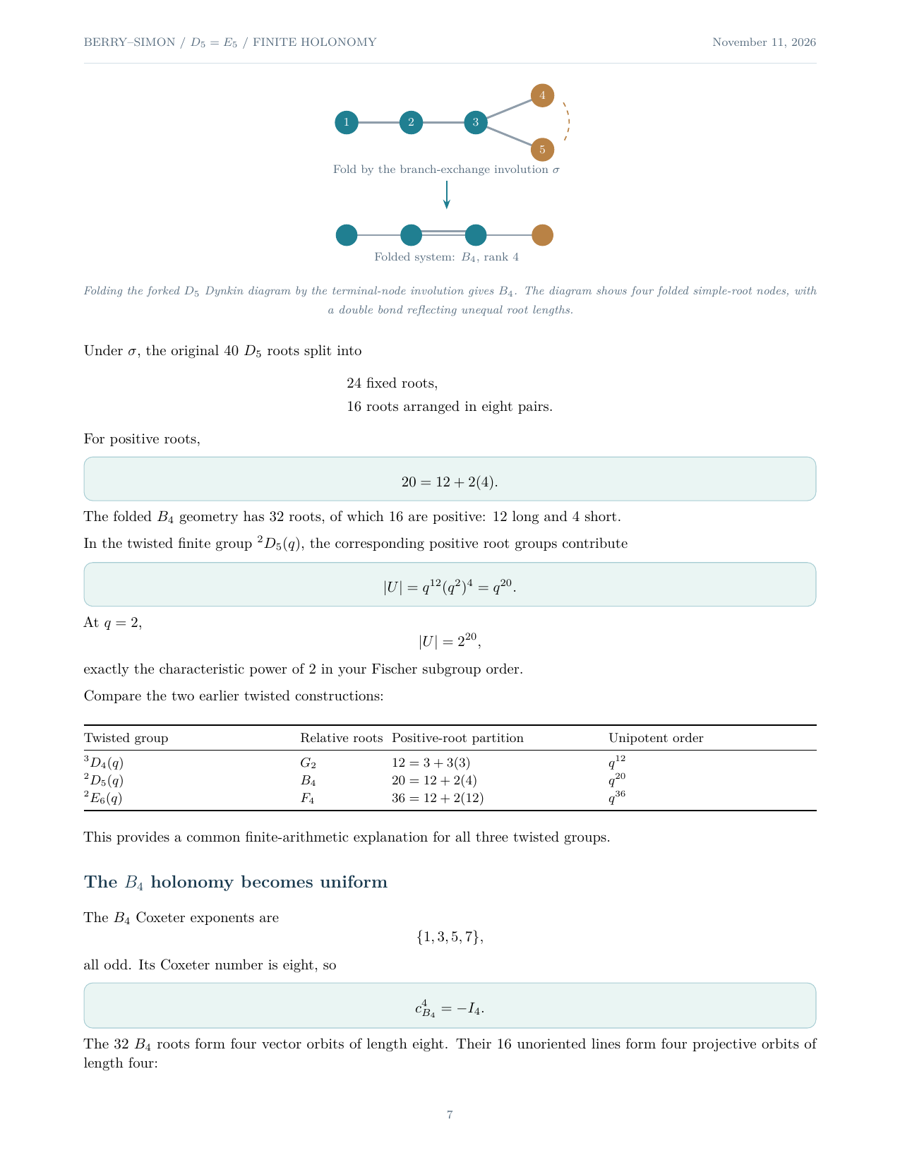
Under \(\sigma\), the original 40 \(D_5\) roots split into

For positive roots,

The folded \(B_4\) geometry has 32 roots, of which 16 are positive: 12 long and 4 short.

In the twisted finite group \({}^2D_5(q)\), the corresponding positive root groups contribute

At \(q = 2\),

exactly the characteristic power of 2 in your Fischer subgroup order.

Compare the two earlier twisted constructions:

Twisted group	Relative roots	Positive-root partition	Unipotent order
\({}^3D_4(q)\)	\(G_2\)	\(12 = 3 + 3(3)\)	\(q^{12}\)
\({}^2D_5(q)\)	\(B_4\)	\(20 = 12 + 2(4)\)	\(q^{20}\)
\({}^2E_6(q)\)	\(F_4\)	\(36 = 12 + 2(12)\)	\(q^{36}\)

This provides a common finite-arithmetic explanation for all three twisted groups.

The \(B_4\) holonomy becomes uniform

The \(B_4\) Coxeter exponents are

all odd. Its Coxeter number is eight, so

The 32 \(B_4\) roots form four vector orbits of length eight. Their 16 unoriented lines form four projective orbits of length four:

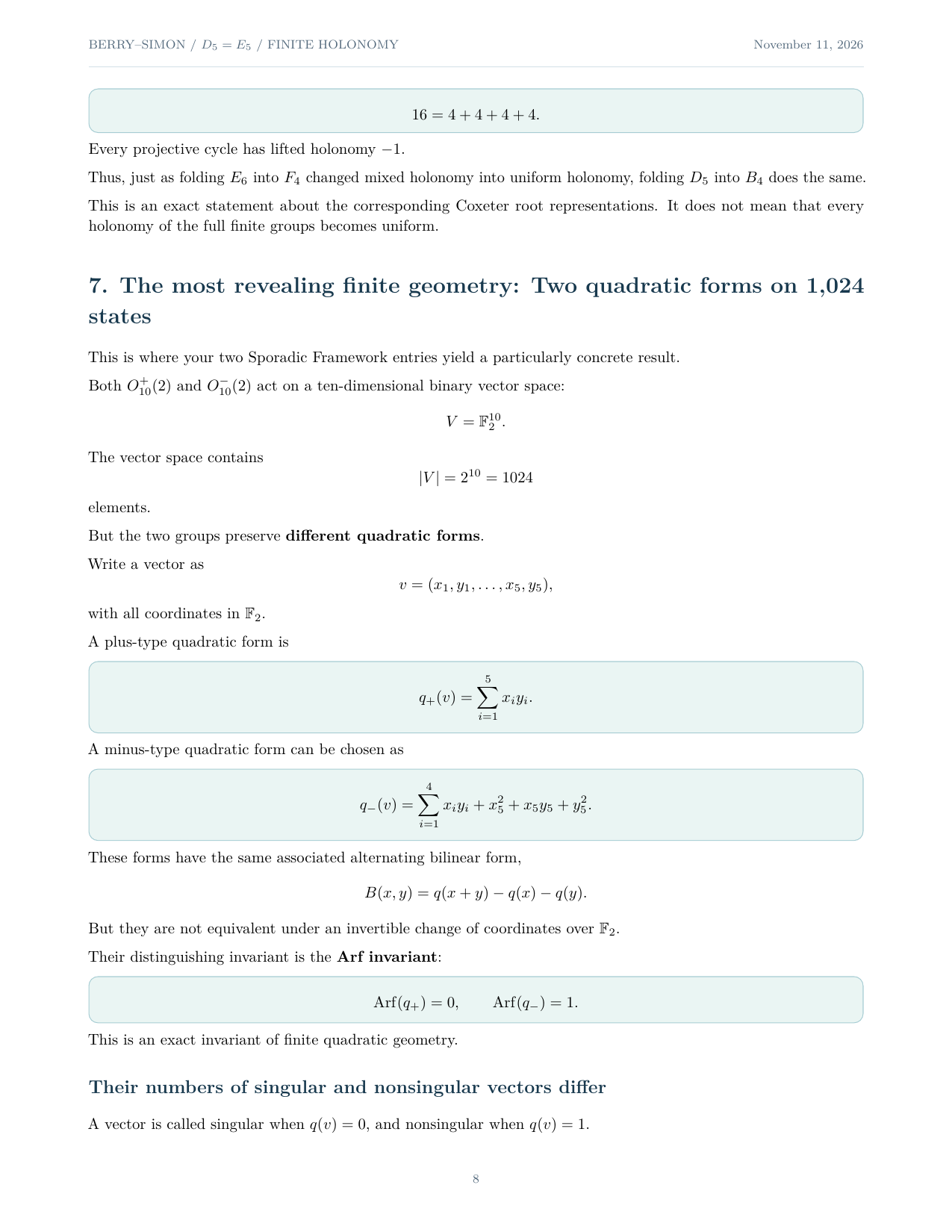
Every projective cycle has lifted holonomy \(-1\).

Thus, just as folding \(E_6\) into \(F_4\) changed mixed holonomy into uniform holonomy, folding \(D_5\) into \(B_4\) does the same.

This is an exact statement about the corresponding Coxeter root representations. It does not mean that every holonomy of the full finite groups becomes uniform.

7. The most revealing finite geometry: Two quadratic forms on 1,024 states

This is where your two Sporadic Framework entries yield a particularly concrete result.

Both \(O_{10}^{+}(2)\) and \(O_{10}^{-}(2)\) act on a ten-dimensional binary vector space:

The vector space contains

elements.

But the two groups preserve different quadratic forms.

Write a vector as

with all coordinates in \(\mathbb{F}_2\).

A plus-type quadratic form is

A minus-type quadratic form can be chosen as

These forms have the same associated alternating bilinear form,

But they are not equivalent under an invertible change of coordinates over \(\mathbb{F}_2\).

Their distinguishing invariant is the Arf invariant:

This is an exact invariant of finite quadratic geometry.

Their numbers of singular and nonsingular vectors differ

A vector is called singular when \(q(v) = 0\), and nonsingular when \(q(v) = 1\).

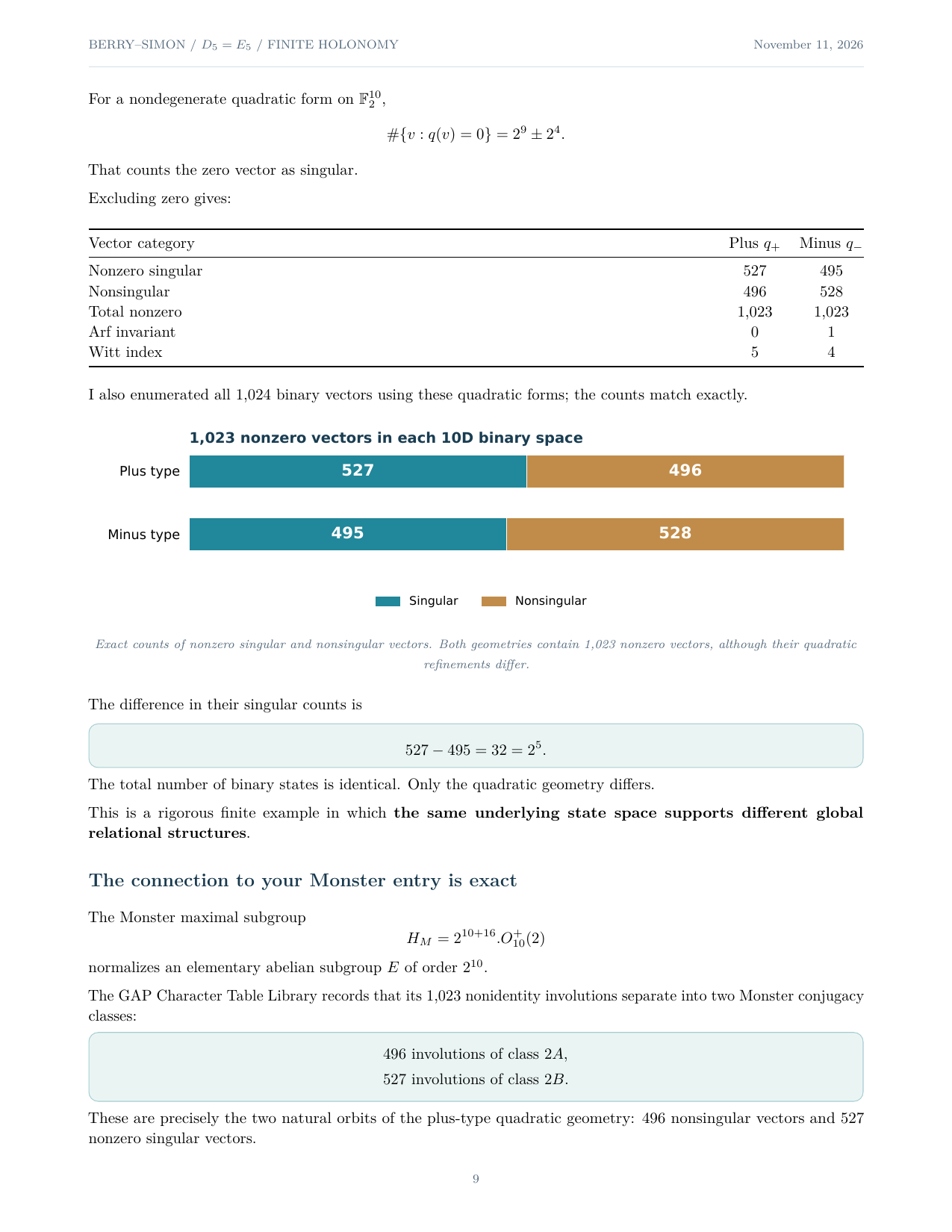
For a nondegenerate quadratic form on \(\mathbb{F}_2^{10}\),

That counts the zero vector as singular.

Excluding zero gives:

Vector category	Plus \(q_+\)	Minus \(q_-\)
Nonzero singular	527	495
Nonsingular	496	528
Total nonzero	1,023	1,023
Arf invariant	0	1
Witt index	5	4

I also enumerated all 1,024 binary vectors using these quadratic forms; the counts match exactly.

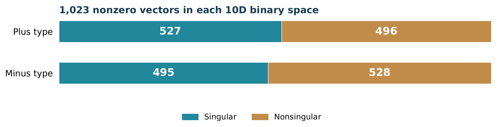
The difference in their singular counts is

The total number of binary states is identical. Only the quadratic geometry differs.

This is a rigorous finite example in which the same underlying state space supports different global relational structures.

The connection to your Monster entry is exact

The Monster maximal subgroup

normalizes an elementary abelian subgroup \(E\) of order \(2^{10}\).

The GAP Character Table Library records that its 1,023 nonidentity involutions separate into two Monster conjugacy classes:

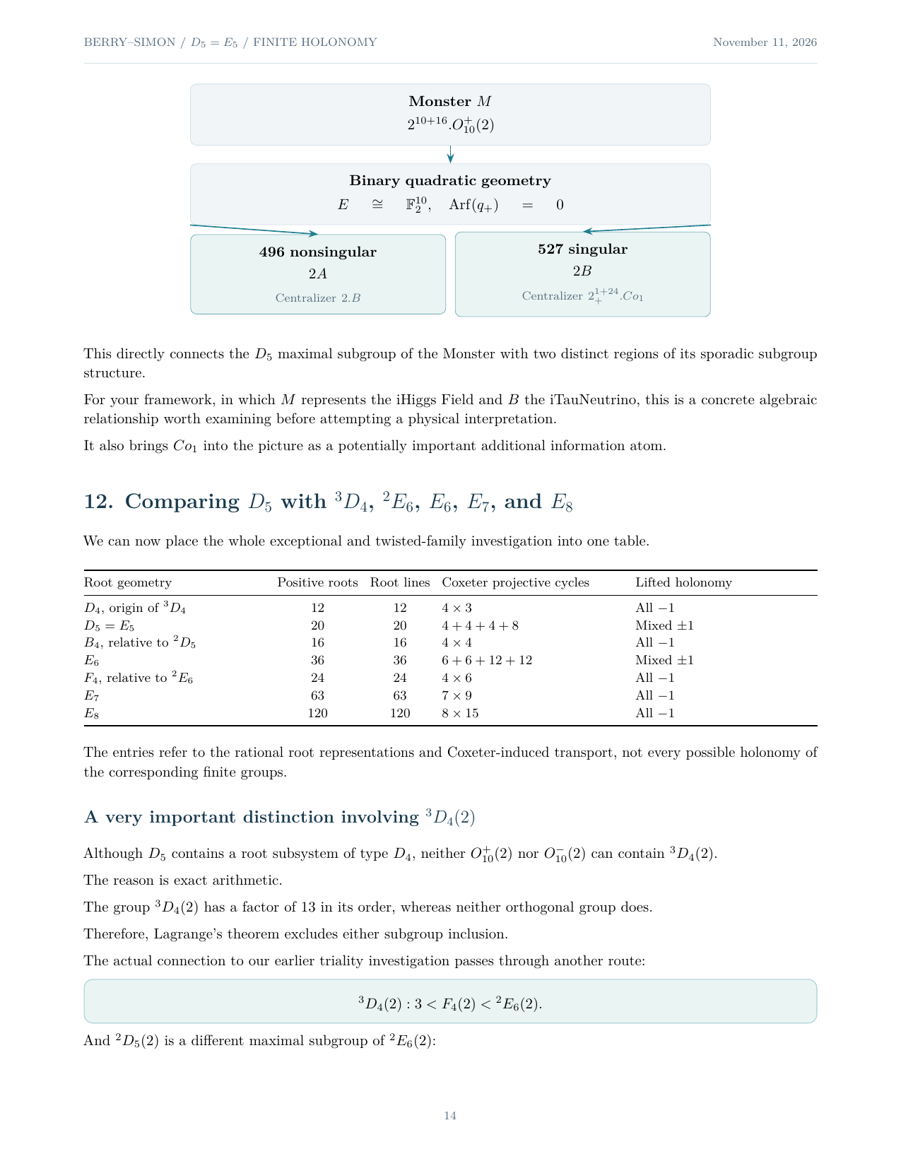
These are precisely the two natural orbits of the plus-type quadratic geometry: 496 nonsingular vectors and 527 nonzero singular vectors.

This is much stronger than observing that your Monster maximal subgroup contains a factor of \(2^{10}\).

It shows that the plus-type quadratic form actually organizes involutions inside the Monster into distinct conjugacy classes.

For the minus-type group in \(Fi_{24}^{\prime}\), the corresponding intrinsic orthogonal geometry has the 495/528 split. That is an exact fact about the natural \(O_{10}^{-}(2)\)-module, though it should not be interpreted as a statement about the Fischer group’s involution classes without an additional embedding calculation.

8. A finite alternative to curvature: Quadratic refinements and incidence

In differential geometry, one often starts with a metric and differentiates it to construct curvature.

Here we can begin with exact finite objects.

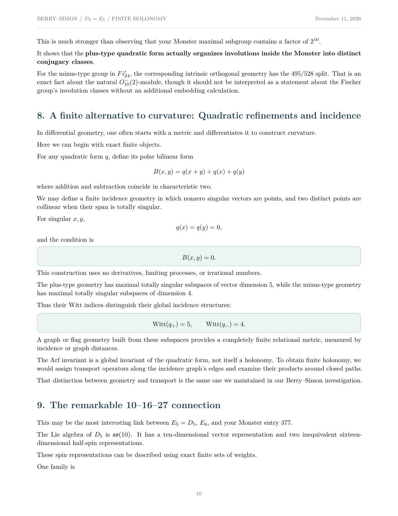
For any quadratic form \(q\), define its polar bilinear form

where addition and subtraction coincide in characteristic two.

We may define a finite incidence geometry in which nonzero singular vectors are points, and two distinct points are collinear when their span is totally singular.

For singular \(x, y\),

and the condition is

This construction uses no derivatives, limiting processes, or irrational numbers.

The plus-type geometry has maximal totally singular subspaces of vector dimension 5, while the minus-type geometry has maximal totally singular subspaces of dimension 4.

Thus their Witt indices distinguish their global incidence structures:

A graph or flag geometry built from these subspaces provides a completely finite relational metric, measured by incidence or graph distances.

The Arf invariant is a global invariant of the quadratic form, not itself a holonomy. To obtain finite holonomy, we would assign transport operators along the incidence graph’s edges and examine their products around closed paths.

That distinction between geometry and transport is the same one we maintained in our Berry–Simon investigation.

9. The remarkable 10–16–27 connection

This may be the most interesting link between \(E_5 = D_5\), \(E_6\), and your Monster entry 377.

The Lie algebra of \(D_5\) is \(\mathfrak{so}(10)\). It has a ten-dimensional vector representation and two inequivalent sixteen-dimensional half-spin representations.

These spin representations can be described using exact finite sets of weights.

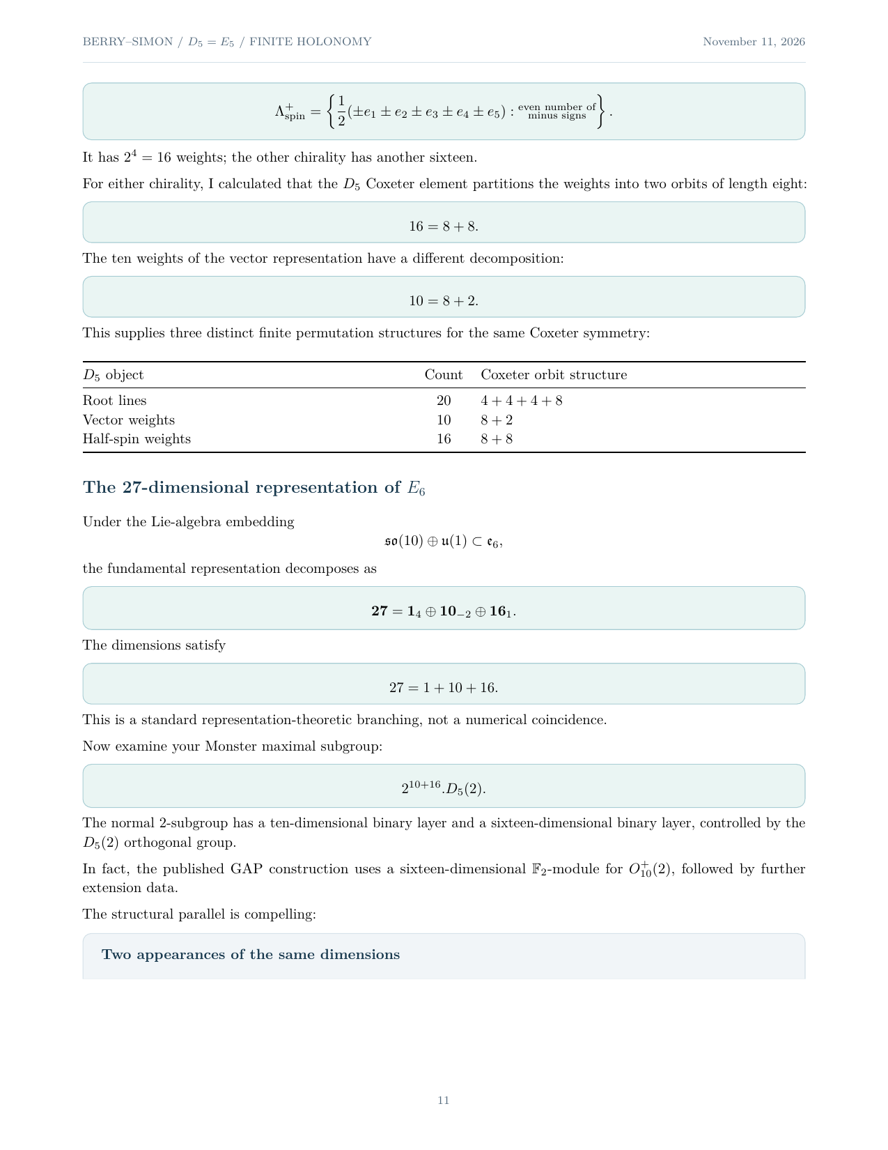
One family is

It has \(2^4 = 16\) weights; the other chirality has another sixteen.

For either chirality, I calculated that the \(D_5\) Coxeter element partitions the weights into two orbits of length eight:

The ten weights of the vector representation have a different decomposition:

This supplies three distinct finite permutation structures for the same Coxeter symmetry:

\(D_5\) object	Count	Coxeter orbit structure
Root lines	20	4+4+4+8
Vector weights	10	8+2
Half-spin weights	16	8+8

The 27-dimensional representation of \(E_6\)

Under the Lie-algebra embedding

the fundamental representation decomposes as

The dimensions satisfy

This is a standard representation-theoretic branching, not a numerical coincidence.

Now examine your Monster maximal subgroup:

The normal 2-subgroup has a ten-dimensional binary layer and a sixteen-dimensional binary layer, controlled by the \(D_5(2)\) orthogonal group.

In fact, the published GAP construction uses a sixteen-dimensional \(\mathbb{F}_2\)-module for \(O_{10}^{+}(2)\), followed by further extension data.

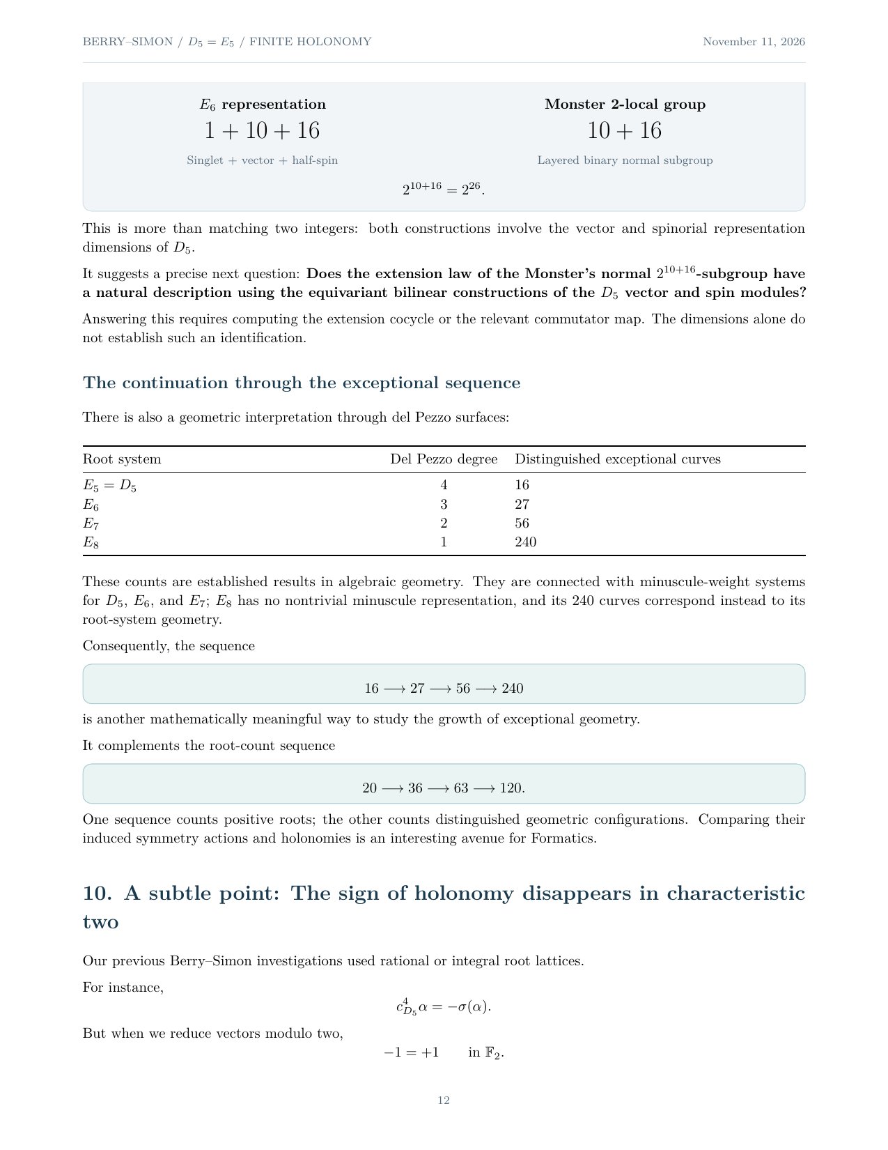
The structural parallel is compelling:

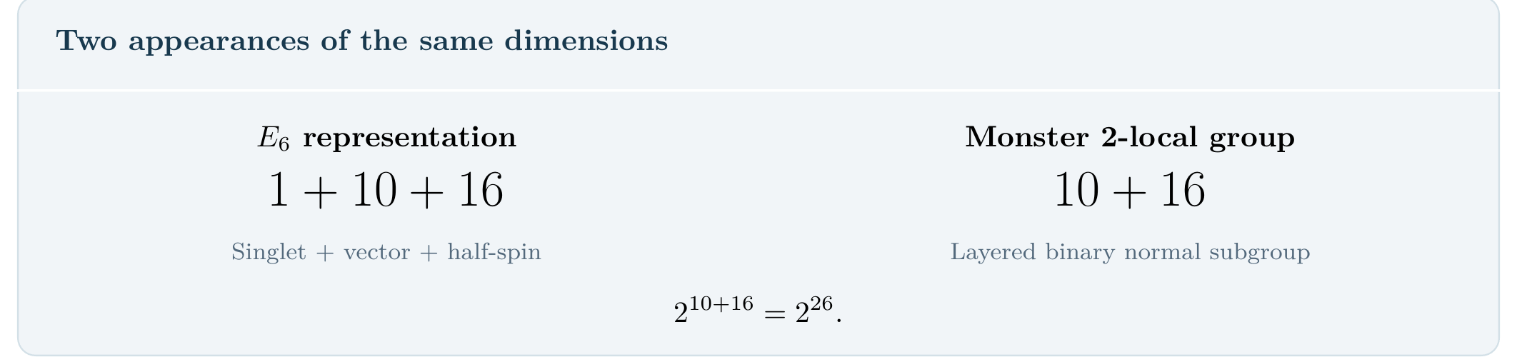
This is more than matching two integers: both constructions involve the vector and spinorial representation dimensions of \(D_5\).

It suggests a precise next question: Does the extension law of the Monster’s normal \(2^{10+16}\)-subgroup have a natural description using the equivariant bilinear constructions of the \(D_5\) vector and spin modules?

Answering this requires computing the extension cocycle or the relevant commutator map. The dimensions alone do not establish such an identification.

The continuation through the exceptional sequence

There is also a geometric interpretation through del Pezzo surfaces:

Root system	Del Pezzo degree	Distinguished exceptional curves
\(E_5 = D_5\)	4	16
\(E_6\)	3	27
\(E_7\)	2	56
\(E_8\)	1	240

These counts are established results in algebraic geometry. They are connected with minuscule-weight systems for \(D_5\), \(E_6\), and \(E_7\); \(E_8\) has no nontrivial minuscule representation, and its 240 curves correspond instead to its root-system geometry.

Consequently, the sequence

is another mathematically meaningful way to study the growth of exceptional geometry.

It complements the root-count sequence

One sequence counts positive roots; the other counts distinguished geometric configurations. Comparing their induced symmetry actions and holonomies is an interesting avenue for Formatics.

10. A subtle point: The sign of holonomy disappears in characteristic two

Our previous Berry–Simon investigations used rational or integral root lattices.

For instance,

But when we reduce vectors modulo two,

Therefore, ordinary sign reversal becomes invisible as a scalar operation:

This is fundamental.

The \(-1\) holonomy of a rational root-line bundle cannot simply be transferred to the binary vector space and expected to remain a distinct phase.

Instead, the binary geometry possesses different invariants:

• The Arf invariant of its quadratic form.
• The Witt index and maximal totally singular subspaces.
• The conjugacy classes of the orthogonal-group transport operators.
• Incidence and closed-path information in the associated finite polar geometry.

Thus, the rational root lattice and the binary orthogonal space provide different kinds of finite information.

The rational model retains an orientation sign. The binary model loses that scalar distinction but retains the distinction between plus-type and minus-type quadratic refinements.

This suggests an important mathematical principle for the Formatic framework:

A finite change of representation may preserve some structural invariants while eliminating others—and may introduce a different set of useful relational invariants.

The corresponding task is to identify exactly which invariants are preserved under each representation map.

11. The Monster’s plus-type geometry leads directly to the Baby Monster and Conway group

The 496/527 division has a remarkable consequence.

Recall that the normal elementary abelian subgroup \(E \cong \mathbb{F}_2^{10}\) of your Monster maximal subgroup contains:

and

The Monster centralizers of these involutions are fundamentally different.

For a class-2A involution \(z_A\),

For a class-2B involution \(z_B\),

Here \(B\) is the Baby Monster and \(Co_1\) is the largest Conway sporadic simple group. The precise relationships, including the intersections with your \(2^{10+16}.O_{10}^{+}(2)\) subgroup, are documented in the GAP calculations.

Thus the plus-type \(D_5\) quadratic geometry distinguishes two families of involutions with different sporadic centralizer structures.

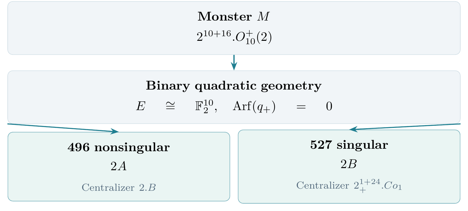
This directly connects the \(D_5\) maximal subgroup of the Monster with two distinct regions of its sporadic subgroup structure.

For your framework, in which \(M\) represents the iHiggs Field and \(B\) the iTauNeutrino, this is a concrete algebraic relationship worth examining before attempting a physical interpretation.

It also brings \(Co_1\) into the picture as a potentially important additional information atom.

12. Comparing \(D_5\) with \({}^3D_4\), \({}^2E_6\), \(E_6\), \(E_7\), and \(E_8\)

We can now place the whole exceptional and twisted-family investigation into one table.

Root geometry	Positive roots	Root lines	Coxeter projective cycles	Lifted holonomy
\(D_4\), origin of \({}^3D_4\)	12	12	\(4\times 3\)	All \(-1\)
\(D_5 = E_5\)	20	20	4+4+4+8	Mixed \(\pm 1\)
\(B_4\), relative to \({}^2D_5\)	16	16	\(4\times 4\)	All \(-1\)
\(E_6\)	36	36	\(6+6+12+12\)	Mixed \(\pm 1\)
\(F_4\), relative to \({}^2E_6\)	24	24	\(4\times 6\)	All \(-1\)
\(E_7\)	63	63	\(7\times 9\)	All \(-1\)
\(E_8\)	120	120	\(8\times 15\)	All \(-1\)

The entries refer to the rational root representations and Coxeter-induced transport, not every possible holonomy of the corresponding finite groups.

A very important distinction involving \({}^3D_4(2)\)

Although \(D_5\) contains a root subsystem of type \(D_4\), neither \(O_{10}^{+}(2)\) nor \(O_{10}^{-}(2)\) can contain \({}^3D_4(2)\).

The reason is exact arithmetic.

The group \({}^3D_4(2)\) has a factor of 13 in its order, whereas neither orthogonal group does.

Therefore, Lagrange’s theorem excludes either subgroup inclusion.

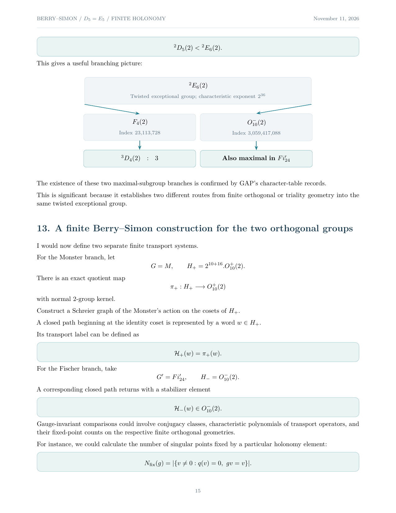
The actual connection to our earlier triality investigation passes through another route:

And \({}^2D_5(2)\) is a different maximal subgroup of \({}^2E_6(2)\):

This gives a useful branching picture:

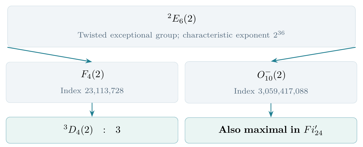
The existence of these two maximal-subgroup branches is confirmed by GAP’s character-table records.

This is significant because it establishes two different routes from finite orthogonal or triality geometry into the same twisted exceptional group.

13. A finite Berry–Simon construction for the two orthogonal groups

I would now define two separate finite transport systems.

For the Monster branch, let

There is an exact quotient map

with normal 2-group kernel.

Construct a Schreier graph of the Monster’s action on the cosets of \(H_+\).

A closed path beginning at the identity coset is represented by a word \(w \in H_+\).

Its transport label can be defined as

For the Fischer branch, take

A corresponding closed path returns with a stabilizer element

Gauge-invariant comparisons could involve conjugacy classes, characteristic polynomials of transport operators, and their fixed-point counts on the respective finite orthogonal geometries.

For instance, we could calculate the number of singular points fixed by a particular holonomy element:

This defines an exact integer-valued relational invariant.

The two constructions would have different initial state spaces and stabilizers. We should not assume they are naturally isomorphic.

What makes this Berry–Simon-like?

In Simon’s geometric interpretation, a quantum state can traverse a closed path in a parameter space and return with nontrivial information recorded in its fiber.

Here, a coset state traverses a closed path and returns with an element of a finite stabilizer group.

The result is discrete holonomy—not necessarily quantum Berry phase.

The mathematical analogy becomes stronger if we can construct a compatible family of spectral projectors and derive the transport from them, rather than assigning it independently.

14. The Formatics synthesis: From root information to quadratic form and holonomy

The central idea now appears to involve at least two different kinds of global information.

The first is structural form information, such as

The second is transport information, such as

Neither determines the other in general.

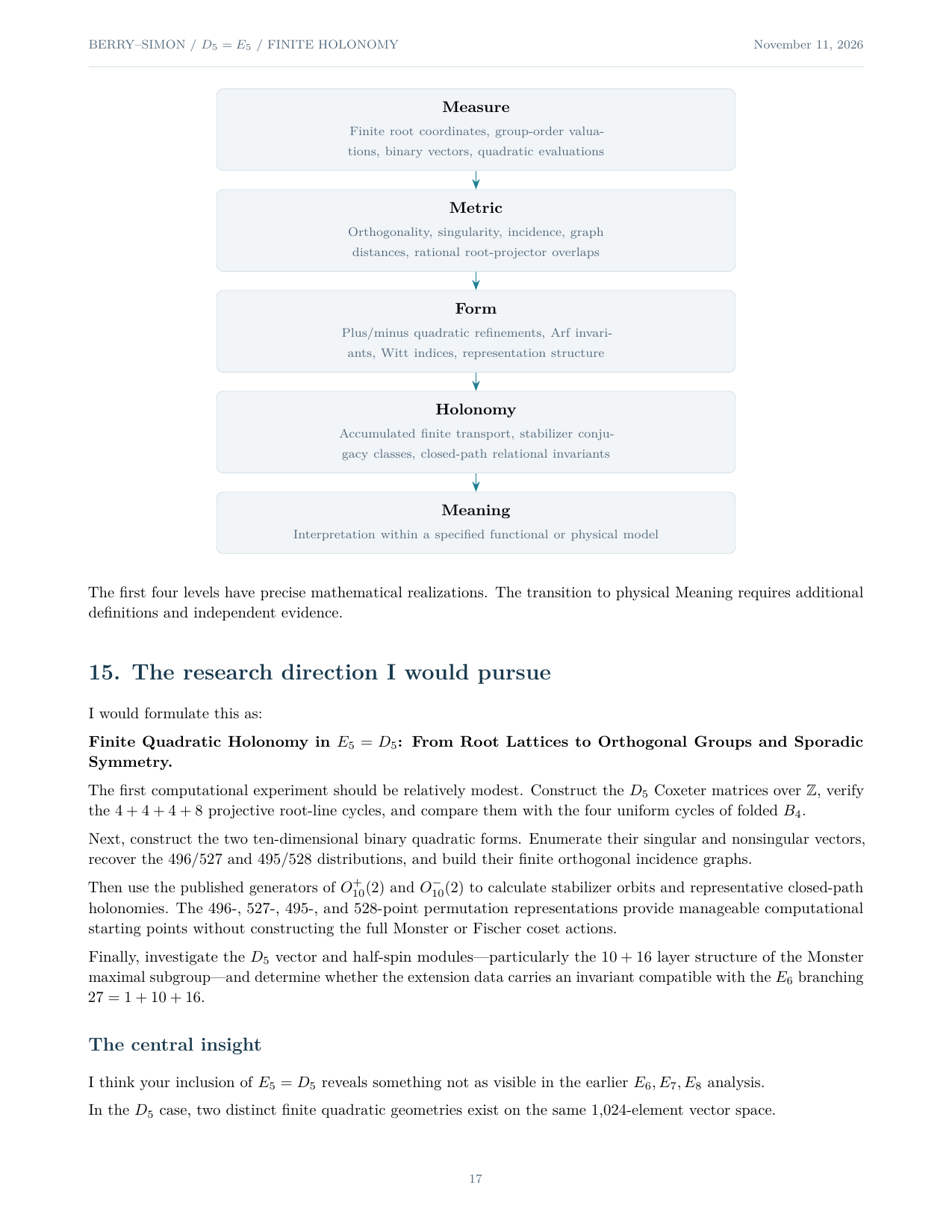
For your Fundamentals of Measure and Meaning, I would explore:

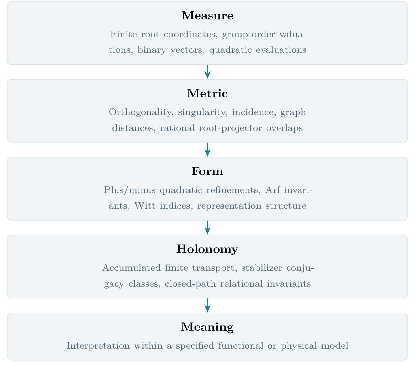
The first four levels have precise mathematical realizations. The transition to physical Meaning requires additional definitions and independent evidence.

15. The research direction I would pursue

I would formulate this as:

Finite Quadratic Holonomy in \(E_5 = D_5\): From Root Lattices to Orthogonal Groups and Sporadic Symmetry.

The first computational experiment should be relatively modest. Construct the \(D_5\) Coxeter matrices over \(\mathbb{Z}\), verify the \(4 + 4 + 4 + 8\) projective root-line cycles, and compare them with the four uniform cycles of folded \(B_4\).

Next, construct the two ten-dimensional binary quadratic forms. Enumerate their singular and nonsingular vectors, recover the 496/527 and 495/528 distributions, and build their finite orthogonal incidence graphs.

Then use the published generators of \(O_{10}^{+}(2)\) and \(O_{10}^{-}(2)\) to calculate stabilizer orbits and representative closed-path holonomies. The 496-, 527-, 495-, and 528-point permutation representations provide manageable computational starting points without constructing the full Monster or Fischer coset actions.

Finally, investigate the \(D_5\) vector and half-spin modules—particularly the \(10 + 16\) layer structure of the Monster maximal subgroup—and determine whether the extension data carries an invariant compatible with the \(E_6\) branching \(27 = 1 + 10 + 16\).

The central insight

I think your inclusion of \(E_5 = D_5\) reveals something not as visible in the earlier \(E_6\), \(E_7\), \(E_8\) analysis.

In the \(D_5\) case, two distinct finite quadratic geometries exist on the same 1,024-element vector space.

Their underlying dimension, cardinality, and polar bilinear form can be identical, yet their Arf invariants, Witt indices, incidence geometries, and orthogonal groups differ.

That is a concrete example of different global structures arising from the same finite local state space.

And in your Sporadic Group Framework, those differences are represented by actual maximal subgroups of the Monster and \(Fi_{24}^{\prime}\).

The potentially important mathematical development is that finite holonomy is only one part of the story. Finite quadratic form itself provides a rigorous invariant of global structure—and \(E_5 = D_5\) gives us a way to investigate both together.

Original document

Download the complete original PDF: The Berry–Simon Connection VI (18 pages, 565 KB)

Show page-by-page facsimile of the original PDF (18 pages)